Colour Autocorrection
Preparing
First of all we should prepare Python infrastructure:
numpyfor array computing.cv2for reading images.matplotlib.pyplotfor plotting results.histogramsit's my own code, you can find it here.
import numpy as np
import cv2
import math

from IPython.display import IFrame

%matplotlib inline
import matplotlib.pyplot as plt

from histograms import *

plt.style.use('seaborn-dark')
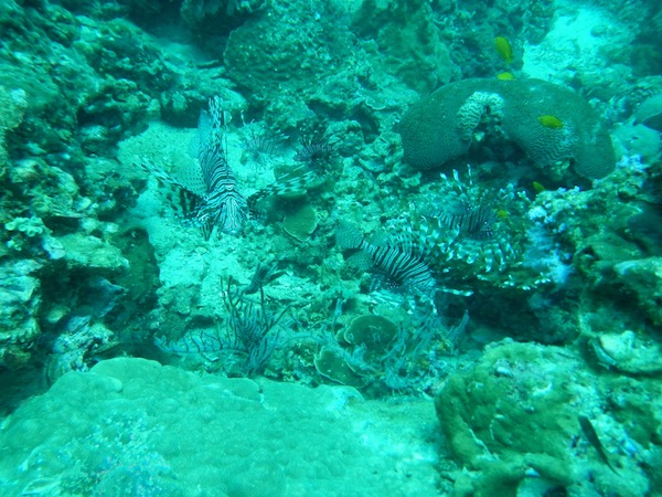
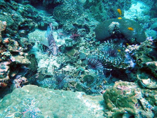
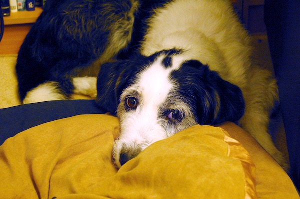
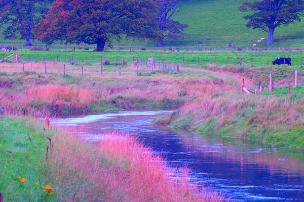
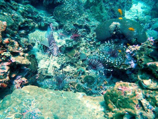
Then we read foreground and background images. As cv2.IMREAD_UNCHANGED mode is used for reading PNG as is with its transparency. Also read image is converted here to float within a range of values [0; 1].
Then channels R and B must be swaped because OpenCV storage images in BGR mode:
img = cv2.imread("photo1.jpg", cv2.IMREAD_UNCHANGED).astype(np.float) / 255.0
img = img[...,[2, 1, 0]]
The Main Idea
The main idea of the proposed approach is channel wise normalisation of histogram and gamma correction with parameters, calculated from the histogram. Assume that the average colour of an image with true white balance and good exposure should be average grey. Moreover, all channels should be represented by the whole range of possible values ([0; 255] for 8-bit image).
Firstly let's try to implement that process manually. So we start with histogram normalisation:
min_val = np.array([0.0, 40.0 / 255, 40.0 / 255])
max_val = np.array([60.0 / 255, 1.0, 0.9])
img_norm = img.copy()
img_norm[...,:] = (img_norm[...,:] - min_val) / (max_val - min_val)
img_norm = np.clip(img_norm, 0.0, 1.0)
Now our image has whole ranges for each channel.
The next step is channel-wise gamma correction offsets median of histogram to 0.5 point:
img_gamma = img_norm.copy()
img_gamma[...,:] = np.power(img_gamma[...,:], np.exp([-1.0, 0.3, 0.1]))
img_gamma = np.clip(img_gamma, 0.0, 1.0)
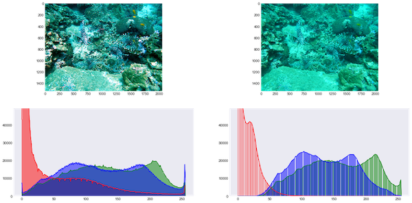
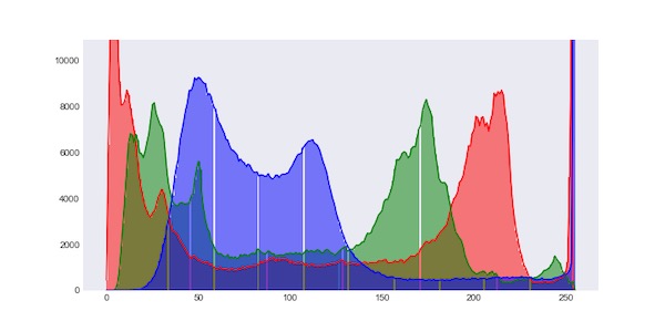
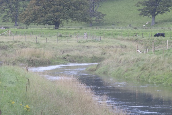
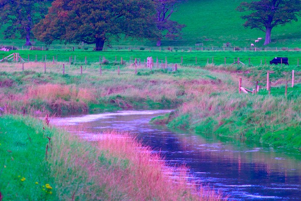
Result image:
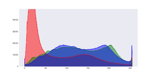
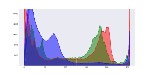
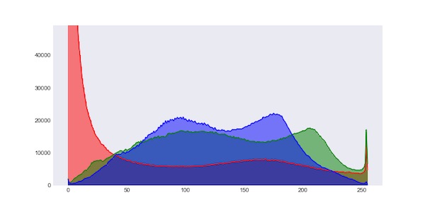
Result image's histogram:
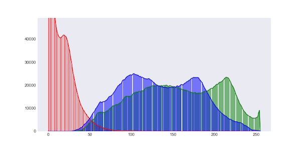
Histogram analysis
What about automatically finding parameters for those adjustments?
img_8 = (img * 255).astype('uint8')
hist_r = cv2.calcHist([img_8], [0], None, [256], [0, 256]).ravel()
hist_g = cv2.calcHist([img_8], [1], None, [256], [0, 256]).ravel()
hist_b = cv2.calcHist([img_8], [2], None, [256], [0, 256]).ravel()
Firstly we should find edges of histogram values:
def find_min_max(hist, threshold=0):
    min_val = 256
    max_val = 0
    for i, v in enumerate(hist):
        if v > threshold:
            if min_val == 256:
                min_val = i
            max_val = i
    return min_val, max_val
edges_r = find_min_max(hist_r)
edges_g = find_min_max(hist_g)
edges_b = find_min_max(hist_b)

min_val = np.array([edges_r[0] / 255.0, edges_g[0] / 255.0, edges_b[0] / 255.0])
max_val = np.array([edges_r[1] / 255.0, edges_g[1] / 255.0, edges_b[1] / 255.0])
img_norm = img.copy()
img_norm[...,:] = (img_norm[...,:] - min_val) / (max_val - min_val)
img_norm = np.clip(img_norm, 0.0, 1.0)
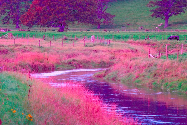
From the result above we can realise that using 0 as a threshold can't make a correct result. So let's try to use some threshold (for example 1% from maximal value) when finding edges.
edges_r = find_min_max(hist_r, max(hist_r) * 0.01)
edges_g = find_min_max(hist_g, max(hist_g) * 0.01)
edges_b = find_min_max(hist_b, max(hist_b) * 0.01)

min_val = np.array([edges_r[0] / 255.0, edges_g[0] / 255.0, edges_b[0] / 255.0])
max_val = np.array([edges_r[1] / 255.0, edges_g[1] / 255.0, edges_b[1] / 255.0])
img_norm = img.copy()
img_norm[...,:] = (img_norm[...,:] - min_val) / (max_val - min_val)
img_norm = np.clip(img_norm, 0.0, 1.0)
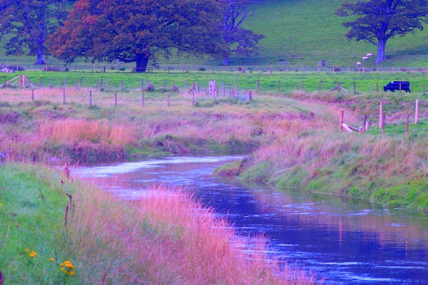
The result with the threshold is much better.
Now we should find a median index in the histogram and offset it to 0.5 point.
def find_median_idx(hist):
    half_total = np.sum(hist) * 0.5
    acc_sum = 0
    for i in range(len(hist)):
        acc_sum += hist[i]
        if acc_sum > half_total:
            return i
    return len(hist) / 2
norm_img_8 = (img_norm * 255).astype('uint8')

norm_hist_r = cv2.calcHist([norm_img_8], [0], None, [256], [0, 256]).ravel()
norm_hist_g = cv2.calcHist([norm_img_8], [1], None, [256], [0, 256]).ravel()
norm_hist_b = cv2.calcHist([norm_img_8], [2], None, [256], [0, 256]).ravel()

med_r = find_median_idx(norm_hist_r) / 255.0
med_g = find_median_idx(norm_hist_g) / 255.0
med_b = find_median_idx(norm_hist_b) / 255.0

img_gamma = img_norm.copy()
img_gamma[...,:] = np.power(img_gamma[...,:], np.exp([(med_r - 0.5) * 2.0, (med_g - 0.5) * 2.0, (med_b - 0.5) * 2.0]))
img_gamma = np.clip(img_gamma, 0.0, 1.0)
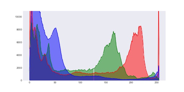
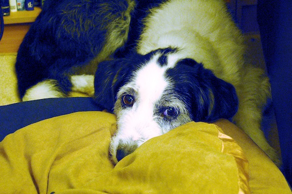
Result image:
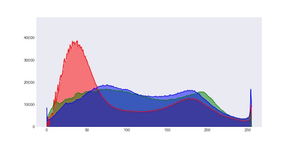
Result image's histogram:
Additional threshold
We used horisontal threshold of histogram values and got good results.
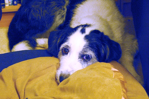
Some images have extremely dark (black) and bright (white) areas. They pull median and edge values over. To prevent that we can use horizontal edges ignoring too bright and too dark pixels.
Below is a function that implemented a fix of that problem:
def auto_correct_v2(img, btm_threshold=0.01, side_threshold=0.01):
    img_8 = (img * 255).astype('uint8')
    hist_r = cv2.calcHist([img_8], [0], None, [256], [0, 256]).ravel()
    hist_g = cv2.calcHist([img_8], [1], None, [256], [0, 256]).ravel()
    hist_b = cv2.calcHist([img_8], [2], None, [256], [0, 256]).ravel()

    hist_r = hist_r[int(255 * side_threshold):int(256 * (1.0 - side_threshold))]
    hist_g = hist_g[int(255 * side_threshold):int(256 * (1.0 - side_threshold))]
    hist_b = hist_b[int(255 * side_threshold):int(256 * (1.0 - side_threshold))]

    edges_r = find_min_max(hist_r, max(hist_r) * btm_threshold)
    edges_g = find_min_max(hist_g, max(hist_g) * btm_threshold)
    edges_b = find_min_max(hist_b, max(hist_b) * btm_threshold)

    min_val = np.array([edges_r[0] / float(len(hist_r)),
                        edges_g[0] / float(len(hist_g)),
                        edges_b[0] / float(len(hist_b))])
    max_val = np.array([edges_r[1] / float(len(hist_r)),
                        edges_g[1] / float(len(hist_g)),
                        edges_b[1] / float(len(hist_b))])

    min_val = min_val * (1.0 - 2.0 * side_threshold) + side_threshold
    max_val = max_val * (1.0 - 2.0 * side_threshold) + side_threshold

    img_norm = img.copy()
    img_norm[...,:] = (img_norm[...,:] - min_val) / (max_val - min_val)
    img_norm = np.clip(img_norm, 0.0, 1.0)


    norm_img_8 = (img_norm * 255).astype('uint8')
    norm_hist_r = cv2.calcHist([norm_img_8], [0], None, [256], [0, 256]).ravel()
    norm_hist_g = cv2.calcHist([norm_img_8], [1], None, [256], [0, 256]).ravel()
    norm_hist_b = cv2.calcHist([norm_img_8], [2], None, [256], [0, 256]).ravel()

    norm_hist_r = norm_hist_r[int(255 * side_threshold):int(256 * (1.0 - side_threshold))]
    norm_hist_g = norm_hist_g[int(255 * side_threshold):int(256 * (1.0 - side_threshold))]
    norm_hist_b = norm_hist_b[int(255 * side_threshold):int(256 * (1.0 - side_threshold))]

    med_r = find_median_idx(norm_hist_r) / len(norm_hist_r)
    med_g = find_median_idx(norm_hist_g) / len(norm_hist_g)
    med_b = find_median_idx(norm_hist_b) / len(norm_hist_b)

    med_r = med_r * (1.0 - 2 * side_threshold) + side_threshold
    med_g = med_g * (1.0 - 2 * side_threshold) + side_threshold
    med_b = med_b * (1.0 - 2 * side_threshold) + side_threshold

    img_gamma = img_norm.copy()
    img_gamma[...,:] = np.power(img_gamma[...,:], np.exp([(med_r - 0.5) * 2.0, (med_g - 0.5) * 2.0, (med_b - 0.5) * 2.0]))
    img_gamma = np.clip(img_gamma, 0.0, 1.0)

    return img_gamma
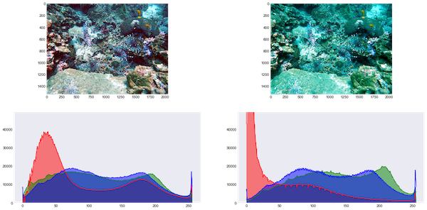
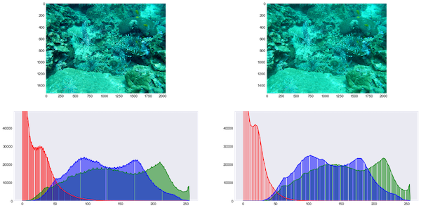
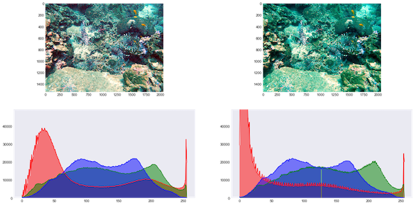
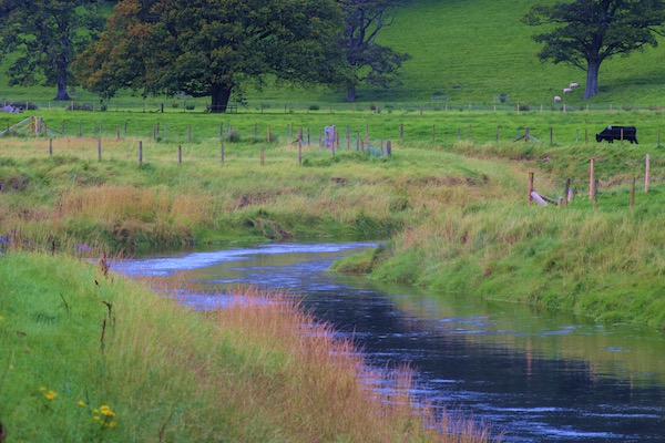
Below is comparing both of versions (left is the 1st):
Ignoring black and white areas we prevent pulling of blue median too much. So the second version is free from some artefacts and softer.
Custom gamma correction
Earlier we use gamma correction fun ction based on the exponent:
g(x, a) = pow(x, exp(a)).
That function has problems in areas near 0 and 1. So I finded alternative function (green):
def custom_gamma(img, b):
    c = 6.5
    a = np.power(c, np.array(b) * 2.0 - 1.0)
    f = 1.0 - np.power(1.0 - img[...,:], 1.0 / a)
    g = np.power(img[...,:], a)
    return (f + g) * 0.5
def auto_correct_v3(img, btm_threshold=0.01, side_threshold=0.01):
    img_8 = (img * 255).astype('uint8')
    hist_r = cv2.calcHist([img_8], [0], None, [256], [0, 256]).ravel()
    hist_g = cv2.calcHist([img_8], [1], None, [256], [0, 256]).ravel()
    hist_b = cv2.calcHist([img_8], [2], None, [256], [0, 256]).ravel()

    hist_r = hist_r[int(255 * side_threshold):int(256 * (1.0 - side_threshold))]
    hist_g = hist_g[int(255 * side_threshold):int(256 * (1.0 - side_threshold))]
    hist_b = hist_b[int(255 * side_threshold):int(256 * (1.0 - side_threshold))]

    edges_r = find_min_max(hist_r, max(hist_r) * btm_threshold)
    edges_g = find_min_max(hist_g, max(hist_g) * btm_threshold)
    edges_b = find_min_max(hist_b, max(hist_b) * btm_threshold)

    min_val = np.array([edges_r[0] / float(len(hist_r)),
                        edges_g[0] / float(len(hist_g)),
                        edges_b[0] / float(len(hist_b))])
    max_val = np.array([edges_r[1] / float(len(hist_r)),
                        edges_g[1] / float(len(hist_g)),
                        edges_b[1] / float(len(hist_b))])

    min_val = min_val * (1.0 - 2.0 * side_threshold) + side_threshold
    max_val = max_val * (1.0 - 2.0 * side_threshold) + side_threshold

    img_norm = img.copy()
    img_norm[...,:] = (img_norm[...,:] - min_val) / (max_val - min_val)
    img_norm = np.clip(img_norm, 0.0, 1.0)


    norm_img_8 = (img_norm * 255).astype('uint8')
    norm_hist_r = cv2.calcHist([norm_img_8], [0], None, [256], [0, 256]).ravel()
    norm_hist_g = cv2.calcHist([norm_img_8], [1], None, [256], [0, 256]).ravel()
    norm_hist_b = cv2.calcHist([norm_img_8], [2], None, [256], [0, 256]).ravel()

    norm_hist_r = norm_hist_r[int(255 * side_threshold):int(256 * (1.0 - side_threshold))]
    norm_hist_g = norm_hist_g[int(255 * side_threshold):int(256 * (1.0 - side_threshold))]
    norm_hist_b = norm_hist_b[int(255 * side_threshold):int(256 * (1.0 - side_threshold))]

    med_r = find_median_idx(norm_hist_r) / len(norm_hist_r)
    med_g = find_median_idx(norm_hist_g) / len(norm_hist_g)
    med_b = find_median_idx(norm_hist_b) / len(norm_hist_b)

    med_r = med_r * (1.0 - 2 * side_threshold) + side_threshold
    med_g = med_g * (1.0 - 2 * side_threshold) + side_threshold
    med_b = med_b * (1.0 - 2 * side_threshold) + side_threshold

    img_gamma = img_norm.copy()
    med = [med_r, med_g, med_b]
    img_gamma = custom_gamma(img_gamma, med)
    img_gamma = np.clip(img_gamma, 0.0, 1.0)

    return img_gamma
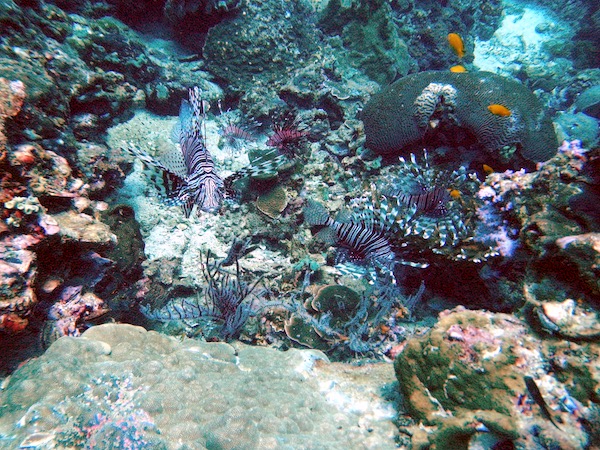
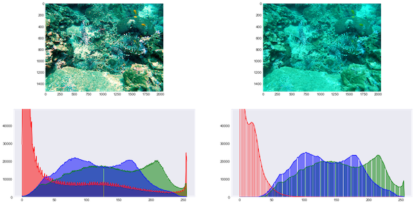
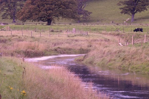
Below are results of using that function against previous version (v2 vs v3):
Other colour spaces
Below are several examples of using that approach for images in other colour spaces. Maybe it makes some new idea in your head how it can be used.
HSV (preserving Hue):
XYZ:
YCrCb:
Lab:
Luv:
YUV:
Combination
From results above we can see that using (H)SV autocorrection we can improve saturation of an image.
Below is a cascade combines RGB+(H)S(V)+RGB autocorrections. While RGB correction uses the 3rd version with custom gamma, HSV uses the 2nd version as softer. Moreover I use a 0.5 amount for saturation to decrease artifacts appearance.
def auto_correct_comb(img):
    k = 0.5
    img_t = img.copy()
    img_rgb_tuned = auto_correct_v3(img_t)

    img_hsv = cv2.cvtColor((img_rgb_tuned[...,[2, 1, 0]] * 255).astype('uint8'), cv2.COLOR_BGR2HSV)
    img_hsv = img_hsv.astype('float') / 255.0
    img_hsv_hue = img_hsv[...,0]
    img_hsv_saturation = img_hsv[...,1]
    img_hsv_value = img_hsv[...,2]
    img_hsv_tuned = auto_correct_v2(img_hsv)
    img_hsv_tuned[...,0] = img_hsv_hue
    img_hsv_tuned[...,1] = img_hsv_tuned[...,1] * (1.0 - k) + img_hsv_saturation * k
    img_hsv_tuned[...,2] = img_hsv_value
    img_tuned = cv2.cvtColor((img_hsv_tuned * 255).astype('uint8'), cv2.COLOR_HSV2BGR)


    img_rgb_tuned = auto_correct_v3(img_tuned[...,[2, 1, 0]].astype('float') / 255.0)

    return img_rgb_tuned
Result image:
Result image's histogram:
Conclusion
So using the provided approach you can automatically correct white balance and exposure of your image. But note, that it can make a worse image as result because a good image is a subjective enough thing.
You can find a snippet implemented that article here.